Profile PyTorch Memory Across Batch Sizes: A Tutorial
A PyTorch model that trains at batch size 8 can fail at batch size 16 without any change in parameter count. The cause is usually not the weights. It is activation storage, allocator behavior, temporary tensors, optimizer state, and memory fragmentation.
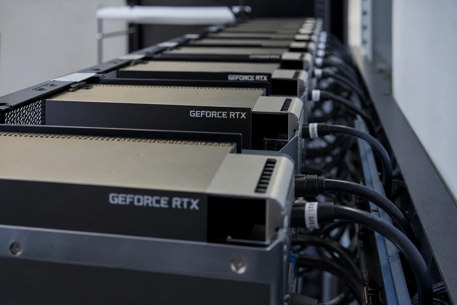
This pytorch tutorial treats GPU memory as a measured property, not an assumption. The target is narrow: profile memory across batch sizes, separate actual tensor allocation from cached reservation, identify operator-level spikes with the PyTorch Profiler, and evaluate whether Automatic Mixed Precision changes the feasible batch-size frontier.
Distinguishing allocated and reserved memory in PyTorch
PyTorch reports several memory quantities. They are not interchangeable. Confusing them leads to incorrect capacity estimates and false conclusions about model footprint.
torch.cuda.memory_allocated() returns the current GPU memory occupied by tensors. This is the active tensor footprint. torch.cuda.max_memory_allocated() returns the peak allocated memory since the beginning of the program or since the peak counter was reset. This is normally the first number to inspect when comparing batch sizes.
torch.cuda.memory_reserved() reports memory held by the PyTorch CUDA caching allocator. Reserved memory is often higher than allocated memory because PyTorch keeps blocks for reuse rather than returning them immediately to the driver. That behavior reduces allocation overhead. It also makes naive readings of GPU memory misleading.
A minimal interpretation table is useful before any profiling script is written.
| Metric | What it measures | Correct interpretation | Common failure |
|---|---|---|---|
memory_allocated() | Current bytes occupied by tensors | Active tensor footprint at a point in execution | Treating it as peak training memory |
max_memory_allocated() | Peak tensor allocation since reset | Best scalar for batch-size comparison | Forgetting to reset before each run |
memory_reserved() | Bytes held by PyTorch allocator | Allocator cache plus active allocations | Calling it “used by the model” |
| Profiler memory events | Operator-level allocation and release | Localizes spikes to layers or operations | Assuming all spikes are parameters |
The distinction is not cosmetic. A model may show 7.2 GB allocated and 10.4 GB reserved. The first number describes tensors. The second describes allocator state. Only the first should be used as the direct model-memory footprint. The second still matters because it affects whether the process can satisfy later allocation requests without fragmentation or additional reservation.
Reserved memory is allocator behavior. Allocated memory is tensor footprint. A memory audit that merges them has already lost precision.
For batch-size profiling, the peak allocated value is usually the main dependent variable. Reserved memory remains a secondary diagnostic. It can expose fragmentation, cache growth, and non-obvious allocator dynamics, especially after repeated trials inside one Python process.
Implementing memory tracking with CUDA stats
A defensible experiment isolates each batch size. The measurement window must start after model construction and before the forward pass. Otherwise, parameter allocation, CUDA context initialization, and warm-up artifacts contaminate the comparison.
The procedure is stable:
1. Move the model to CUDA.
2. Run one optional warm-up iteration if the objective is steady-state measurement.
3. Clear gradients with set_to_none=True.
4. Reset PyTorch peak-memory counters using torch.cuda.reset_peak_memory_stats().
5. Synchronize CUDA before and after the measured region using torch.cuda.synchronize().
6. Run forward pass, loss computation, backward pass, and optimizer step if training memory is the target.
7. Record memory_allocated(), max_memory_allocated(), and memory_reserved().
The measured region must match the question. Inference profiling should not include backward pass. Training profiling should include backward pass and optimizer step, because gradients and optimizer states are part of the operational footprint.
A compact measurement loop can be described without ambiguity:
- For each batch size in
[1, 2, 4, 8, 16, 32], allocate synthetic input with the same shape and dtype used in production. - Reset the peak counter immediately before the measured pass.
- Use
torch.cuda.synchronize()to prevent asynchronous kernels from shifting measurements across boundaries. - Store peak allocated bytes and reserved bytes after the pass.
- Convert bytes to MiB or GiB only for reporting. Keep raw bytes in logs.
The key implementation detail is counter reset. Without it, max_memory_allocated() retains the highest value observed earlier in the process. A batch-size sweep then becomes monotonic by construction, even if the later measurements are smaller. That is not profiling. It is state leakage.
A practical logging row should contain at least these fields:
| Field | Reason |
|---|---|
| Batch size | Independent variable under test |
| Input shape | Prevents invalid comparisons between tasks |
| Precision mode | FP32, AMP, BF16, or FP16 changes activation footprint |
| Peak allocated bytes | Main memory-pressure metric |
| Reserved bytes | Allocator cache and fragmentation diagnostic |
| Step time | Memory reduction that destroys throughput may be a bad trade |
| OOM flag | Necessary for estimating the feasible frontier |
The experiment should not be run with changing sequence lengths, dynamic padding, or data augmentation that alters tensor shapes unless those variables are explicitly part of the test. For transformer workloads, sequence length can dominate batch size. For vision workloads, image resolution has the same role. A batch-size sweep is only interpretable when the other dimensions are controlled.
Profiling operator-level memory with PyTorch Profiler
CUDA stats provide scalar measurements. They do not identify the operation that caused the spike. The PyTorch Profiler fills that gap. Since the modern profiler became available in PyTorch 1.8+, it has been the standard native tool for tracing CPU and CUDA activity, including memory events.
The profiler should be used after the coarse batch-size sweep has identified an interesting region. Profiling every candidate batch size is usually unnecessary and adds overhead. The better pattern is to profile three points:
1. A clearly safe batch size.
2. The largest batch size that completes.
3. The smallest batch size that fails or approaches the memory limit, if the run can be instrumented without aborting the process.
The profiler can record memory activity per operator. In practice, the useful question is not “how much memory does the model use,” but “which operations allocate transient tensors large enough to move the run into failure.” Attention blocks, large matrix multiplications, normalization paths, and loss computation can each create temporary allocations that do not appear as parameters.
A profiler trace should be inspected for:
- Operators with large self CUDA memory allocation.
- Operators that allocate repeatedly inside loops.
- Unexpected dtype promotions from FP16 or BF16 to FP32.
- Tensor reshapes that create copies rather than views.
- Concatenation patterns that allocate large contiguous buffers.
- Activation-heavy layers whose cost scales with batch size and sequence length.
For readers who need broader scientific context around machine learning systems without implementation detail, a general science and technology explainer can be useful. The profiler, however, is not an explainer. It is an instrument. Its output should be treated as a trace of allocation events, not as a narrative about model quality.
The profiler has overhead. It should not be used to report final throughput unless the overhead is separately quantified. Its function in this tutorial is localization. CUDA memory counters provide the batch-size curve. The profiler explains anomalies in that curve.
The profiler is not the primary metric. It is the microscope used after the scalar measurement shows a lesion.
Analyzing memory scaling patterns across batch sizes
In training, memory normally contains a fixed component and a batch-dependent component. The fixed component includes model weights and optimizer state. The variable component includes activations and temporary tensors. For many architectures, activation memory scales approximately linearly with batch size across a stable region.
The model can be represented as:
peak_memory(batch) ≈ fixed_overhead + batch_size × activation_slope
This is a useful approximation, not a law. Very small batch sizes can be dominated by CUDA context and allocator behavior. Very large batch sizes can encounter fragmentation, workspace changes, or kernel selection effects. Dynamic shapes can break the relation entirely.
A batch-size sweep should therefore be interpreted through slopes, not isolated points. If peak allocated memory moves from 4.1 GB at batch size 4 to 6.3 GB at batch size 8 and 10.7 GB at batch size 16, the activation slope is visible. If the curve jumps irregularly, the profiler should be used to inspect operator-level allocations at the discontinuity.
A representative reporting table should include both raw memory and scaling behavior.
| Batch size | Peak allocated | Reserved | Increment vs previous | Interpretation |
|---|---|---|---|---|
| 1 | 2.6 GB | 3.1 GB | — | Fixed overhead dominates |
| 2 | 3.0 GB | 3.6 GB | +0.4 GB | Low activation contribution |
| 4 | 3.9 GB | 4.8 GB | +0.9 GB | Scaling becomes visible |
| 8 | 5.8 GB | 7.0 GB | +1.9 GB | Near-linear region |
| 16 | 9.7 GB | 11.4 GB | +3.9 GB | Activation cost dominates |
| 32 | OOM | OOM | — | Capacity exceeded |
The values above are illustrative. They should not be reused as expected memory for a particular architecture. A BERT encoder, a diffusion U-Net, and a decoder-only transformer with long context length will not share the same curve. The method transfers. The numbers do not.
Several patterns are common in real traces.
Linear allocated memory with larger reserved memory
This is the healthy baseline. max_memory_allocated() grows predictably with batch size. memory_reserved() stays above it because the caching allocator retains blocks. The gap is not a defect by itself.
The action is simple: select the largest batch size with adequate headroom. A production training job should not run at the exact measured limit. Data variability, validation passes, checkpointing, and occasional temporary allocations can exceed the benchmark path.
Sudden jump at one batch size
A discontinuity indicates that something changed. It may be kernel workspace selection. It may be an internal operation that crosses a threshold. It may be a tensor copy introduced by a shape-dependent branch.
The profiler should be run at the batch size immediately before and after the jump. If a single operator accounts for the new allocation, optimization can be targeted. If many operators increase proportionally, the jump may simply reflect activation growth combined with allocator block size behavior.
Reserved memory grows while allocated memory remains stable
This is often allocator cache behavior or fragmentation. It can happen in repeated experiments inside one process. The correct response is not to claim that the model footprint increased. The allocated peak is the tensor measurement.
For clean benchmarking, batch sizes can be executed in separate processes. That removes cross-trial allocator state. It also produces more reproducible capacity estimates when measuring near the OOM boundary.
Small batch sizes show poor efficiency
Batch size 1 or 2 often has high memory per sample because fixed overhead dominates. This is not surprising. Parameter memory, optimizer state, CUDA context, and framework overhead are amortized over too few samples.
This matters when comparing two implementations. A model that looks inefficient at batch size 1 may become competitive at batch size 16 if its activation slope is lower. Conversely, a parameter-efficient architecture can still fail at larger batches if its activation path is expensive.
Training memory is not inference memory
A common error is to profile inference and extrapolate to training. The two regimes have different memory structures.
Inference can often discard intermediate activations earlier. Training must retain activations needed for backward computation unless activation checkpointing is used. Training also introduces gradients and optimizer state. For Adam-like optimizers, optimizer states can be a material fixed cost relative to the weights.
The measurement script should therefore expose mode explicitly.
| Component | Inference | Training |
|---|---|---|
| Model parameters | Present | Present |
| Forward activations | Limited lifetime | Retained for backward |
| Gradients | Absent | Present |
| Optimizer state | Absent | Present after optimizer initialization |
| Backward temporary tensors | Absent | Present |
| Peak memory location | Often forward path | Often backward path |
For a code implementation article, this distinction is operational. The same model object can produce a low inference footprint and a much larger training peak. A repository that reports only inference memory has not characterized training feasibility.
Gradient accumulation also requires careful language. It can emulate a larger effective batch size by performing multiple smaller micro-batches before an optimizer step. It does not make a large physical batch fit into memory. The peak activation footprint remains tied to the micro-batch size, not the accumulated batch size.
This is often the correct engineering solution when the optimizer requires a larger effective batch for stability but the GPU cannot hold it in one pass. The memory profile should label both terms: micro-batch size and effective batch size.
Optimizing footprint with Automatic Mixed Precision
Automatic Mixed Precision reduces memory pressure by using lower-precision formats for selected operations. In PyTorch, AMP through torch.cuda.amp commonly uses FP16 where appropriate while preserving FP32 where numerical stability requires it. The expected memory reduction for eligible tensors can approach 2x, but the end-to-end reduction is smaller when fixed FP32 components remain.
The correct experiment compares FP32 and AMP under the same batch-size sweep. The measurement window, input shape, optimizer, and model mode must remain constant. Only precision mode changes.
A useful AMP comparison table looks like this:
| Batch size | FP32 peak allocated | AMP peak allocated | Result |
|---|---|---|---|
| 4 | Completes | Completes | AMP lowers footprint |
| 8 | Completes | Completes | Throughput comparison required |
| 16 | Near limit | Completes | AMP expands feasible range |
| 32 | OOM | Near limit or OOM | Architecture-dependent |
The claim should remain conservative. AMP can significantly reduce activation memory. It does not halve every component of training memory. Optimizer states may remain FP32. Some operations run in FP32. Temporary buffers can still dominate local peaks. Numerical stability must also be monitored through loss scaling and validation metrics.
AMP should be evaluated with the same profiler workflow. If peak memory barely changes, the model may be dominated by FP32 states, non-AMP operations, or allocator behavior. If peak memory falls but step time worsens, the implementation may be bottlenecked elsewhere. Memory optimization is not automatically throughput optimization.
A reproducible batch-size profiling protocol
A minimal protocol for serious implementation work has four passes.
First, run a dry initialization pass. This loads the model, creates optimizer state if training, initializes CUDA context, and removes one-time startup effects from the measured run.
Second, run the scalar sweep. Measure max_memory_allocated() and memory_reserved() for each batch size. Use controlled input shapes. Reset peak stats before each measurement. Synchronize around the measured region.
Third, profile selected batch sizes with torch.profiler. Inspect memory events per operator. Focus on discontinuities and near-limit configurations.
Fourth, repeat the sweep with AMP. Compare not only memory but also step time and failure boundary.
The output should be a table, not a paragraph of impressions. A practical report might contain:
- Hardware identifier, such as GPU class and memory capacity.
- PyTorch version and CUDA runtime.
- Model name and parameter count if known.
- Input tensor shape and dtype.
- Training or inference mode.
- Optimizer and whether optimizer state was initialized.
- Batch-size list.
- Peak allocated memory.
- Reserved memory.
- Step time.
- OOM status.
- Precision mode.
Parameter count alone is insufficient. Two models with similar parameter counts can have very different activation profiles. A transformer with long sequence length can spend memory in attention activations. A convolutional model can show different scaling behavior with resolution. A diffusion pipeline can shift peaks across U-Net, VAE, and conditioning components. The measurement protocol must follow the actual execution graph.
Limitations and failure cases
This method is empirical, but it is not omniscient. PyTorch memory counters report PyTorch-managed CUDA allocations. External libraries, custom CUDA kernels, and non-PyTorch allocations may not be fully represented in the same way. GPU driver tools can show process-level memory that differs from PyTorch allocated memory. That difference is expected.
The profiler also changes execution characteristics. It records events and adds overhead. It should not be left enabled for final performance reporting unless the profiling overhead is part of the experiment.
OOM handling requires discipline. After an out-of-memory exception, the process may be in a poor state for subsequent measurements. Continuing the same sweep can contaminate later results. A robust harness runs each batch size in a fresh process or stops after the first OOM when measuring a monotonic batch sequence.
Allocator cache behavior can also mislead repeated trials. Calling cache-clearing functions may reduce reserved memory, but it does not change the peak tensor requirement of the model. It can make logs look cleaner. It should not be presented as a model optimization.
Finally, exact overhead differs by architecture and kernel path. The memory profile of a Llama-family decoder, a BERT encoder, or a vision transformer cannot be inferred from generic rules. CUDA kernel versions and GPU architecture may alter fragmentation and workspace behavior. Those details require measurement on the target stack.
Practical conclusion
Profiling PyTorch memory across batch sizes is a controlled measurement problem. The core metric is max_memory_allocated() inside a correctly bounded execution window. memory_reserved() is allocator context, not model footprint. The PyTorch Profiler is used after the scalar sweep to attribute spikes to operators.
The useful result is not a single number. It is a curve: batch size against peak allocated memory, with precision mode, input shape, and training regime held constant. That curve exposes the activation slope, the fixed overhead, the OOM boundary, and the effect of AMP.
For implementation work, this is the difference between guessing a batch size and auditing one. The first fails late. The second fails in a controlled experiment, with enough evidence to change the model, the precision mode, the micro-batch size, or the operator path.