Hugging Face Transformers Library: Performance in Numbers
The Hugging Face Transformers library is no longer only a convenient model-loading layer. It is an execution surface for training and inference across PyTorch, JAX/Flax, TensorFlow, ONNX Runtime, DeepSpeed, and hardware-specific backends.
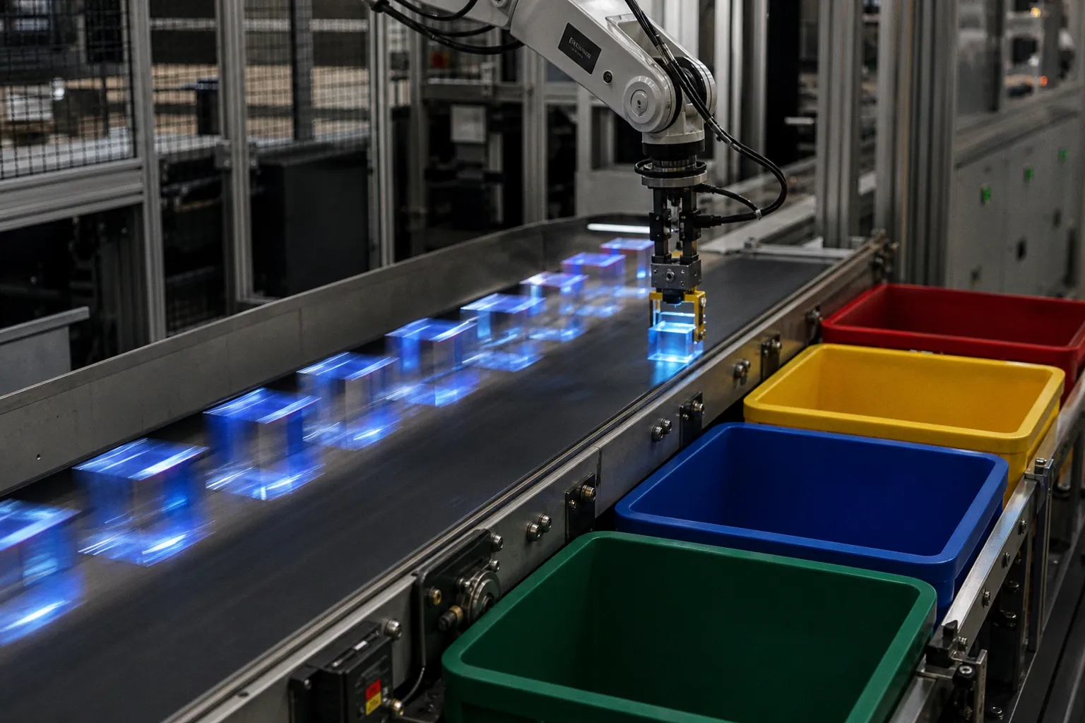
The empirical claim is narrow: the library can reduce memory pressure by roughly 50% with FP16 or BF16 mixed precision, expose distributed training paths through ZeRO stages, and cut inference latency by multiples when SDPA, BetterTransformer, or ONNX Runtime are applicable. The methodology supports that claim only under bounded conditions. Unsupported architectures, small batch sizes, unstable FP16 runs, and export-incompatible operators can erase the headline gains.
Memory Optimization via Mixed Precision and ZeRO Scaling
The first performance constraint in transformer training is usually not raw compute. It is memory residency. Parameters, gradients, optimizer states, activations, temporary buffers, and attention matrices all compete for device memory. The Hugging Face Transformers library addresses this through mixed precision in the Trainer API and through DeepSpeed integration for optimizer and parameter partitioning.
FP16 and BF16 are the blunt instruments. They reduce tensor storage width from 32 bits to 16 bits where the operation permits it. In practical terms, this can reduce memory usage by approximately 50% for the affected tensors and can accelerate training on NVIDIA GPUs with Tensor Cores. The result is not equivalent to a universal 2x speedup. Memory bandwidth, kernel choice, activation checkpointing, dataloader throughput, and communication overhead can dominate.
The distinction between FP16 and BF16 matters. FP16 has a narrower numerical range and often requires gradient scaling to avoid underflow during backpropagation. BF16 preserves the exponent width of FP32 and is generally less fragile, but hardware support is more constrained. A run that is stable in BF16 may require explicit loss scaling or conservative hyperparameters in FP16. Treating “mixed precision” as a single setting is poor benchmarking practice.
DeepSpeed changes the scaling axis. ZeRO stages partition training state across devices:
| Optimization path | What is reduced | Primary benefit | Primary cost |
|---|---|---|---|
| FP16/BF16 mixed precision | Tensor storage width for eligible computation | Lower memory footprint; Tensor Core acceleration | Numerical sensitivity, especially FP16 |
| ZeRO-1 | Optimizer states | Lower per-GPU optimizer memory | Added communication |
| ZeRO-2 | Optimizer states and gradients | Larger effective batch and model capacity | More synchronization complexity |
| ZeRO-3 | Optimizer states, gradients, and parameters | Enables training of models above 100B parameters on distributed clusters | Highest orchestration and communication overhead |
ZeRO-3 is the relevant boundary case. It partitions parameters themselves across GPUs. This makes very large models trainable by avoiding full parameter replication on every device. The trade-off is predictable. Parameter shards must be materialized or communicated when needed. The cluster fabric becomes part of the model architecture in operational terms. NVLink, InfiniBand, PCIe topology, and overlap between communication and computation determine whether theoretical capacity becomes useful throughput.
Memory optimization is not free capacity. It is capacity purchased with numerical risk, communication overhead, or both.
For applied implementation work, the error is to benchmark only successful throughput. Failed or unstable runs are also data. FP16 overflow, divergence after warmup, or a small but repeatable degradation in validation metrics belongs in the performance report. The hugging face transformers library provides the switches. It does not remove the obligation to run an ablation study on precision mode, batch size, gradient accumulation, and optimizer partitioning.
A minimal empirical protocol should isolate four variables:
1. Baseline FP32 throughput and peak memory. This establishes whether training is compute-bound or memory-bound before optimization.
2. FP16 and BF16 runs with identical seeds and schedules. The comparison should include loss curves, validation metrics, and instability events, not only examples per second.
3. ZeRO stage sweep. ZeRO-1, ZeRO-2, and ZeRO-3 should be evaluated separately because their communication profiles differ materially.
4. Effective batch-size control. Gradient accumulation changes optimization dynamics. It should not be confused with pure memory optimization.
The measurable output should include tokens per second, samples per second, peak allocated memory, optimizer state memory, communication time where observable, and final task metric. Without the final metric, a faster run may only be a faster failed experiment.
Accelerating Inference with BetterTransformer and SDPA
Inference performance in transformer models is dominated by attention, matrix multiplication, memory access patterns, and framework overhead. BetterTransformer targets this path by using PyTorch’s scaled dot product attention, exposed through torch.nn.functional.scaled_dot_product_attention. In supported architectures, this can provide faster inference and lower memory consumption. Reported gains can reach roughly 2x to 4x depending on sequence length and workload.
The condition is important. SDPA acceleration is sensitive to sequence length. Short sequences often spend a larger share of time in dispatch overhead and non-attention layers. Long sequences expose the quadratic cost of attention and therefore give optimized attention kernels more room to matter. Batch size also shifts the result. A latency benchmark at batch size 1 and a throughput benchmark at batch size 32 are not interchangeable.
BetterTransformer is best viewed as a kernel-level and graph-level substitution for supported model families. It is not a semantic model improvement. It should preserve outputs within expected numerical tolerance, but precision mode and backend kernels can change exact floating-point values. This is usually irrelevant for classification or generation metrics at normal tolerances. It is not irrelevant for regression-style evaluation or tests with strict equality assumptions.
A disciplined inference benchmark separates three measurements:
| Measurement | Why it matters | Common failure mode |
|---|---|---|
| First-token latency | Critical for interactive generation | Hidden tokenizer and preprocessing time |
| Tokens per second after prefill | Measures sustained decode throughput | Mixed with batch scheduling artifacts |
| Peak memory during inference | Determines deployable batch and context length | Reported without KV cache accounting |
For encoder-only models, the relevant benchmark is often end-to-end latency at fixed sequence lengths: 128, 512, and possibly 1024 tokens. For decoder-only generation, prefill and decode should be separated. Prefill is parallel across the prompt. Decode is sequential over generated tokens and strongly affected by KV cache layout.
The hugging face transformers code path can look deceptively uniform because model invocation remains similar. The backend execution is not uniform. Eager PyTorch, PyTorch 2.x compilation paths, SDPA, BetterTransformer, quantized runtimes, and ONNX Runtime all operate under different assumptions. A benchmark that lists only the model name and GPU name is underspecified.
Where SDPA Usually Has Leverage
The empirical expectation is strongest under these conditions:
- Longer input sequences. Attention cost becomes a larger fraction of total latency.
- Supported transformer architectures. Unsupported models cannot be assumed to benefit.
- Modern PyTorch and compatible GPU kernels. The accelerated path depends on backend dispatch.
- Inference-heavy workloads. Training introduces additional memory and gradient constraints.
- Batch shapes that are stable. Highly variable sequence lengths reduce the benefit of optimized kernels unless padding and batching are handled carefully.
The negative case is equally important. Small sequence classification jobs may show limited gains because the model is already fast relative to framework and input pipeline overhead. Optimization should then move to batching, tokenization parallelism, memory pinning, and serving architecture rather than attention kernels.
Bridging Research to Production with ONNX Runtime
ONNX Runtime is the main export path when the goal is to reduce Python and framework overhead, apply graph-level optimizations, and move inference toward production serving. For transformer models, ONNX Runtime can apply constant folding, node fusion, and operator-level optimizations. Reported latency reductions often fall in the 2x to 5x range relative to standard PyTorch eager mode, but that comparison is not universal.
The relevant baseline matters. PyTorch eager mode is not the same as PyTorch with compiled graphs, optimized attention kernels, or vendor-specific inference libraries. ONNX Runtime may outperform eager execution substantially and still be close to, below, or above an optimized PyTorch 2.x path on a particular model. The correct claim is conditional: ONNX Runtime can reduce latency materially when export succeeds, graph optimizations apply, and the execution provider is well matched to the hardware.
Export is also an architectural audit. Dynamic axes, unsupported operators, custom model heads, generation loops, and tokenizer-side behavior can complicate the path. Encoder-only classification models tend to export more cleanly than full autoregressive generation stacks with custom decoding logic. The model graph is only part of the serving system. Tokenization, batching, postprocessing, and request scheduling remain outside many simplified ONNX benchmarks.
ONNX export is not a deployment guarantee. It is a graph contract that still has to survive operators, shapes, and serving constraints.
A useful ONNX Runtime evaluation should include the following sequence:
1. Numerical parity check. Compare logits or task outputs against the source PyTorch model within a documented tolerance.
2. Static versus dynamic shape test. Static shapes often benchmark better but may not match production traffic.
3. Execution provider comparison. CPU, CUDA, and vendor-specific providers can produce different bottlenecks.
4. Batch-size sweep. Latency and throughput can move in opposite directions as batch size increases.
5. End-to-end measurement. Include tokenization and postprocessing when the benchmark is intended to represent user-visible latency.
The deployment decision then becomes less ambiguous. If ONNX Runtime cuts model execution latency by 3x but tokenization consumes half the request time, the system-level gain is smaller. If the service is throughput-bound and batchable, the result may still be valuable. If the service is strict p99 latency at batch size 1, the conclusion may differ.
JAX, Flax, and XLA: Throughput by Compilation
The Transformers library also supports JAX primarily through Flax. This path matters because XLA compilation can fuse operations, optimize memory layouts, and generate efficient device-specific programs for TPUs and GPUs. In training loops with stable shapes, XLA can materially improve throughput. The cost is compilation latency and reduced tolerance for dynamic execution patterns.
JAX changes the implementation style. PyTorch code often accepts eager inspection, imperative debugging, and irregular control flow. JAX rewards static shapes, pure functions, explicit state handling, and compilation-friendly loops. The performance ceiling can be high. The engineering surface is less forgiving.
For high-throughput training, the relevant comparison is not “PyTorch versus JAX” in general. It is a controlled test of the same model, dataset pipeline, precision, batch size, and hardware target. XLA compilation can produce strong results when the workload is stable. It can also introduce expensive recompilation when input shapes vary or when Python-side control flow leaks into the training path.
A practical comparison should focus on the following metrics:
| Metric | PyTorch/Trainer path | JAX/Flax/XLA path |
|---|---|---|
| Initial iteration time | Usually lower startup overhead | Can include substantial compilation cost |
| Steady-state throughput | Strong with optimized kernels and mixed precision | Strong when shapes are stable and XLA fuses effectively |
| Debuggability | Easier imperative inspection | More constrained under compilation |
| Shape flexibility | More tolerant in eager mode | More sensitive to recompilation |
| TPU alignment | Possible through supported stacks | Native strategic advantage |
This is where many hugging face model benchmarks lose diagnostic value. They report steady-state throughput after warmup but omit compilation time. For long training runs, compilation overhead may be amortized and irrelevant. For short fine-tuning jobs or iterative experimentation, it can dominate wall-clock productivity. Both numbers should be reported.
The Flax path is therefore best suited to workloads where the training shape is predictable and the execution horizon is long enough to amortize compilation. It is less attractive when the implementation is still under active debugging or when the dataset produces highly variable shapes that trigger recompilation or padding inefficiency.
Hardware-Specific Tuning and Optimum Integration
The Transformers ecosystem increasingly treats hardware-specific execution as a first-class concern. The Optimum library expanded this role by providing optimization interfaces for different backends and accelerators. This is the correct direction. Generic model code is useful for research portability. Production performance requires backend-specific assumptions.
Hardware-specific tuning can include ONNX Runtime acceleration, quantization paths, graph optimization, and accelerator integrations. The value is not that these tools exist. The value is that they reduce the distance between a research checkpoint and an executable artifact with measurable latency, throughput, and memory properties.
Still, hardware-specific tuning introduces benchmark fragmentation. The same model may be tested under several incompatible execution modes:
- PyTorch eager execution with FP32.
- PyTorch mixed precision with FP16 or BF16.
- PyTorch with SDPA or BetterTransformer.
- PyTorch 2.x compiled execution.
- ONNX Runtime with graph optimizations.
- Vendor-specific execution providers.
- JAX/Flax with XLA compilation.
- DeepSpeed training with ZeRO partitioning.
A single leaderboard score cannot summarize these paths. The benchmark must state the execution path, precision, device, driver stack, batch size, sequence length, and whether preprocessing is included. Otherwise, transformers library performance becomes a marketing number rather than an empirical measurement.
The Benchmark Matrix That Actually Separates Signal from Noise
A compact but useful evaluation matrix should not attempt to test every possible combination. It should isolate the optimizations most likely to matter for the target workload.
| Workload | Primary bottleneck | First optimization to test | Secondary optimization |
|---|---|---|---|
| Fine-tuning BERT-style encoder | GPU memory and attention compute | FP16/BF16 mixed precision | SDPA or BetterTransformer if supported |
| Training large decoder model | Model state memory | DeepSpeed ZeRO-2 or ZeRO-3 | Activation checkpointing and tensor parallel strategy |
| Batch inference for embeddings | Throughput and batching | ONNX Runtime or compiled PyTorch | Static shape batching |
| Interactive text generation | First-token latency and decode throughput | SDPA/BetterTransformer if supported | KV cache and serving scheduler tuning |
| TPU training | Compilation and device utilization | Flax/JAX with XLA | Static shapes and input pipeline optimization |
This matrix is not exhaustive. It is a guardrail against arbitrary tuning. Optimization should follow the bottleneck. Applying ZeRO-3 to a model that already fits comfortably on one GPU may reduce throughput because communication overhead exceeds memory benefit. Exporting to ONNX for a model with unstable dynamic shapes may add operational complexity without improving p99 latency. Enabling FP16 without validating loss stability can produce a fast run with corrupted convergence.
Interpreting Transformers Memory Usage Metrics
Transformers memory usage metrics are often misread because they collapse distinct categories into a single peak number. Peak allocated GPU memory is useful, but it does not explain the allocation. A training run can be dominated by activations, optimizer states, gradients, parameters, or temporary attention buffers. Each category has a different remedy.
Mixed precision reduces tensor width for eligible computations. It does not remove optimizer state overhead unless the optimizer implementation also stores states efficiently. ZeRO partitions optimizer states, gradients, and parameters depending on stage. Activation checkpointing reduces stored activations by recomputing them during backward passes. Attention kernel changes can reduce temporary memory during inference. These are not interchangeable techniques.
A correct memory report should include:
1. Peak allocated device memory. The basic capacity indicator.
2. Peak reserved memory. Useful for understanding allocator behavior.
3. Batch size and sequence length. Memory scales sharply with sequence length in attention-heavy workloads.
4. Precision mode. FP32, FP16, and BF16 are not equivalent.
5. Optimizer and ZeRO stage. Optimizer states can dominate training memory.
6. Activation checkpointing status. Recompute changes both memory and runtime.
7. Model architecture and parameter count. Encoder-only, encoder-decoder, and decoder-only models have different profiles.
For inference, KV cache memory must be included for generation workloads. A decoder-only model serving long contexts may fit at prompt time and then fail under generation pressure because cache memory grows with generated length, number of layers, hidden size, and batch size. Reporting only model weight memory is insufficient.
What the Numbers Support
The strongest evidence for the Hugging Face Transformers library is not that it makes every model fast. It is that it exposes several mature optimization mechanisms behind a relatively consistent interface. Mixed precision can roughly halve memory use for eligible tensors and accelerate Tensor Core workloads. DeepSpeed ZeRO stages make distributed training of billion-parameter and above-100B-parameter models feasible when the cluster fabric can absorb communication. BetterTransformer and SDPA can deliver 2x to 4x inference improvements for supported architectures and favorable sequence lengths. ONNX Runtime can produce 2x to 5x latency reductions versus standard PyTorch eager mode when graph optimization and execution providers align.
The limitations are equally material. Not all models support BetterTransformer. ONNX Runtime is not always faster than modern compiled PyTorch paths. FP16 is not always numerically stable without gradient scaling. JAX/XLA can improve steady-state throughput while adding compilation costs and shape constraints. ZeRO-3 can enable scale while reducing per-step efficiency if communication is poorly overlapped.
The practical conclusion is conservative. The hugging face transformers library should be treated as a benchmarking substrate, not as a performance guarantee. Its value is the ability to run controlled ablation studies across precision, partitioning, graph optimization, and backend execution without rewriting the model stack from scratch. The winning configuration is workload-specific. The only defensible result is the one measured on the target architecture, with the target sequence lengths, under the target latency or throughput objective.